Examples#
In the tandem repository you find many examples.
The folders poisson and elasticity contain test problems for the
Poisson and Elasticity solvers.
In the folder tandem you find SEAS models.
The folder options contains PETSc solver configurations.
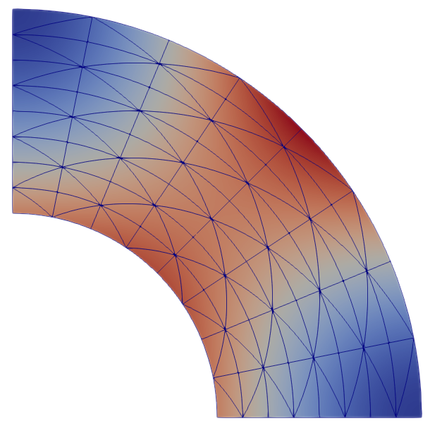
Elasticity problem#
From the build directory, run
$ ./app/static ../examples/elasticity/2d/cosine.toml --output cosine
After a successful run, there should be the file cosine.pvtu in your
build directory.
The pvtu-file can be visualized with ParaView.
Cf. the following visualization of the cosine example:
Along with the pvtu-file, you also get console output, e.g.
Solver warmup: 0.120276 s
Solve: 0.310153 s
Residual norm: 1.20671e-11
Iterations: 127
L2 error: 2.88579e-09
We see that we need quite a number of iterations to solve this problem. Let’s use a LU-decomposition instead of an iterative solver:
$ ./app/static ../examples/elasticity/2d/cosine.toml --output cosine \
      --petsc -options_file ../examples/options/lu_mumps.cfg
The console output should be similar to the following:
Solver warmup: 0.194319 s
Solve: 0.00834613 s
Residual norm: 0
Iterations: 1
L2 error: 2.88579e-09
We see that the warm-up time increased but the solve time decreased a lot. Moreover, we only need 1 “iteration” as we used a direct solver.
Now open up the parameter file, cosine.toml:
resolution = 0.125

[elasticity]
lib = "cosine.lua"
...
The cosine example uses a generated mesh, therefore we can adjust the mesh
resolution in the parameter with the resolution parameter.
You could now edit the parameter file to adjust the resolution.
Alternatively, you can override top-level parameters from the command line:
$ ./app/static ../examples/elasticity/2d/cosine.toml --output cosine \
      --resolution 0.0625 --petsc -options_file ../examples/options/lu_mumps.cfg
You should now see
Solver warmup: 0.760638 s
Solve: 0.0306711 s
Residual norm: 0
Iterations: 1
L2 error: 2.42624e-11
The solve and warm-up time increased considerably, but also the error is lower. Indeed, comparing the errors with
shows that the empirical convergence order is close to the theoretical convergence
order 7. (Assuming that you compiled tandem with POLYNOMIAL_DEGREE=6.)
SEAS problem#
Attention
Please install Gmsh for this section.
On your local machine, go to the folder examples/tandem/2d and run
$ gmsh -2 bp1_sym.geo -setnumber Lf 0.5
You have now created a mesh with an on-fault resolution of 0.5 km. Now go to your build folder (inside the Docker container, if you used Docker) and run:
$ ./app/tandem ../examples/tandem/2d/bp1_sym.toml \
      --petsc -options_file ../examples/options/lu_mumps.cfg \
      -options_file ../examples/options/rk45.cfg
In comparison to the Elasticity example, we added the rk45.cfg options
file which selects an adaptive Runge-Kutta time-stepping scheme.
By default, tandem enables monitoring of time and time-step size in a user-friendly format (values given in year, days, hours, etc.).
The option -ts_monitor enables monitoring of time and time-step size in the default PETSc layout, that is time step and time in seconds.
Finally, the option -disable_custom_ts_monitor allows disable any time step monitoring.
Time to fetch a coffee, as this is going to take a while.
In order to speed things up, add --mode QDGreen:
$ ./app/tandem ../examples/tandem/2d/bp1_sym.toml --mode QDGreen \
      --petsc -options_file ../examples/options/lu_mumps.cfg \
      -options_file ../examples/options/rk45.cfg
Tandem now spends some time in a pre-computation step, but the time-stepping itself will be much faster.
The code logs the slip rate and other quantities at certain points and saves
those in the fltst_* files.
You can view these files using the viewrec tool from the SeisSol project –
even when tandem is still running.